Daily Paper Reading
Topic: latent reasoning + variational Bayes + inference-time computation
Link: http://arxiv.org/abs/2502.01567
 arxiv.org
Latent Thought Models with Variational Bayes Inference-Time ComputationA language model with explicit latent thought vectors, sequence-specific posterior inference, and a fast-slow learning loop.
arxiv.org
Latent Thought Models with Variational Bayes Inference-Time ComputationA language model with explicit latent thought vectors, sequence-specific posterior inference, and a fast-slow learning loop.LTM [1]
Latent Thought Models with Variational Bayes Inference-Time Computation
D. Kong, M. Zhao, D. Xu, B. Pang, S. Wang, E. Honig, Z. Si, C. Li, J. Xie, S. Xie, Y. Wu, (2025)
DOI
assumes that a text sequence \(\mathbf{x}\) is generated not by a plain autoregressive decoder alone, but by an autoregressive decoder conditioned on explicit latent thought vectors \(\mathbf{z}\). These latent vectors are organized by layer, and each decoder layer cross-attends to its corresponding latent thoughts.
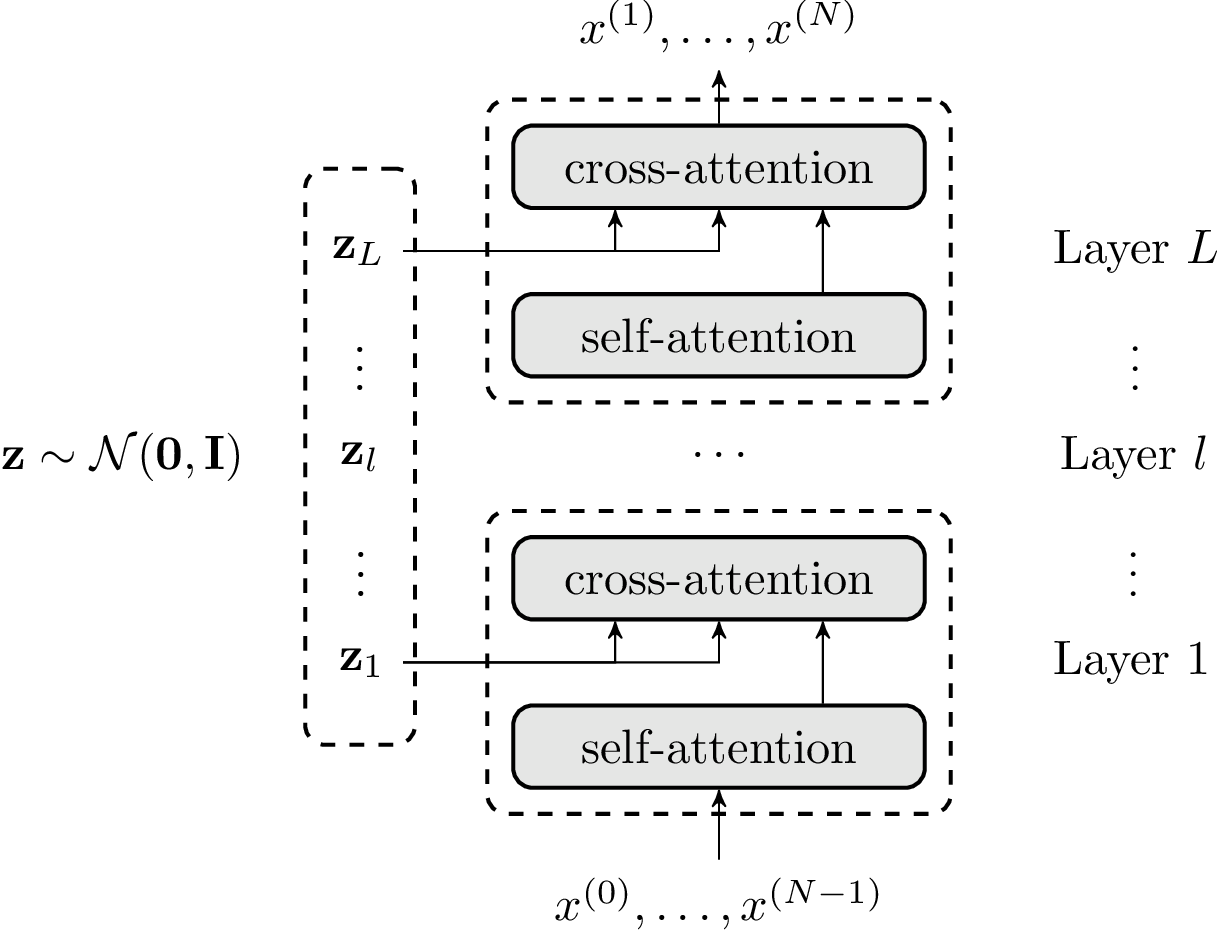
Illustration of the LTM. Latent thought vectors $\mathbf{z}$ ~ N(0, I) are organized by layer, and $\mathbf{z}_l$ is injected into decoder layer l through cross-attention. $\mathbf{z}$ is instance-specific, while $\beta$ is shared globally.
The core loop is:
- Introduce an explicit latent state \(\mathbf{z}\).
- Maintain a sequence-specific posterior \(q(\mathbf{z}\mid\mathbf{x})\).
- Run a finite inner-loop optimization of that posterior during both training and testing.
- Decode tokens autoregressively under the inferred latent state.
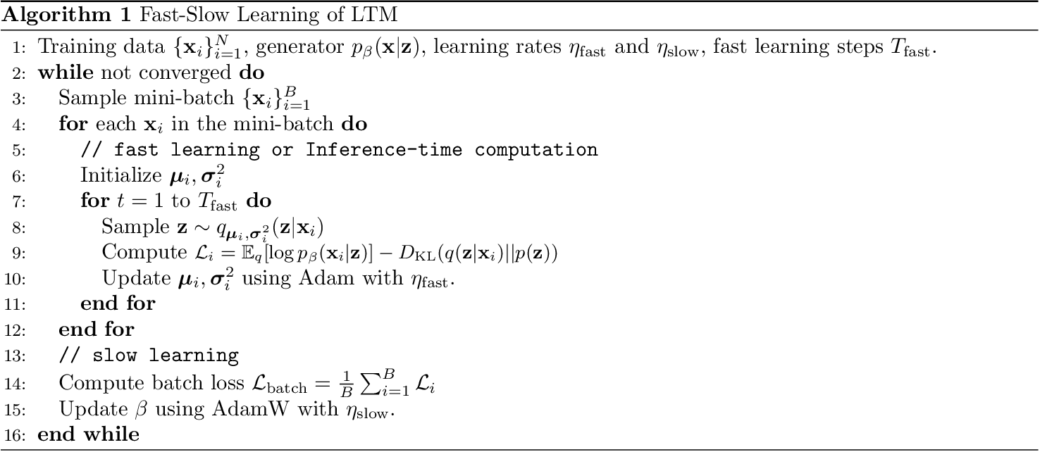
Fast-Slow Learning of LTM. Here p(z) is the prior over latent thought vectors, and the paper uses the isotropic Gaussian prior N(0, I).
Thought-guided autoregressive generation with a constrained context window
Given a sequence $\mathbf{x}$, the thought-guided generator parameterized by $\beta$ is still autoregressive:
$$ p_{\beta}(\mathbf{x}\mid \mathbf{z}) = \prod_{n=1}^{N} p_{\beta}(x_n \mid \mathbf{z}, \mathbf{x}_{1:n-1}). $$The paper further emphasizes a short-context setting:
$$ p_{\beta}(\mathbf{x}\mid \mathbf{z}) = \prod_{n=1}^{N} p_{\beta}(x_n \mid \mathbf{z}, \mathbf{x}_{n-k:n-1}). $$The point is that once the token context window is deliberately shortened, \(\mathbf{z}\) is forced to act as a stronger global information carrier.
Marginal likelihood and posterior inference
The marginal likelihood is
$$ p_{\beta}(\mathbf{x}) = \int p_{\beta}(\mathbf{x}\mid \mathbf{z})\, p(\mathbf{z})\, d\mathbf{z}, \qquad p(\mathbf{z}) = \mathcal{N}(\mathbf{0}, \mathbf{I}). $$Its maximum-likelihood gradient is
$$ \nabla_{\beta}\log p_{\beta}(\mathbf{x}) = \mathbb{E}_{p_{\beta}(\mathbf{z}\mid\mathbf{x})}\left[\nabla_{\beta}\log p_{\beta}(\mathbf{x}\mid\mathbf{z})\right]. $$If one estimates the posterior by sampling, the paper gives the Langevin update
$$ \mathbf{z}^{\tau+1} = \mathbf{z}^{\tau} + s \nabla_{\mathbf{z}} \log p_{\beta}(\mathbf{z}^{\tau}\mid\mathbf{x}) + \sqrt{2s}\,\boldsymbol{\epsilon}^{\tau}, \qquad \boldsymbol{\epsilon}^{\tau}\sim \mathcal{N}(\mathbf{0}, \mathbf{I}). $$The paper also studies a VAE-style amortized inference baseline. Its adopted method, however, is classical variational Bayes: compared with Langevin sampling, it is more efficient; compared with the VAE baseline, it avoids learning a large inference model and mitigates posterior collapse.
classical variational Bayes with the reparameterization trick
What the paper actually uses is this sequence-specific variational posterior
$$ q(\mathbf{z}\mid\mathbf{x}) = \mathcal{N}(\boldsymbol{\mu}, \boldsymbol{\sigma}^{2}). $$and then maximize the evidence lower bound (ELBO):
$$ \mathcal{L}(\beta,\boldsymbol{\mu},\boldsymbol{\sigma}^{2}) = \mathbb{E}_{q(\mathbf{z}\mid\mathbf{x})}\left[\log p_{\beta}(\mathbf{x}\mid\mathbf{z})\right] - \mathrm{KL}\!\left(q(\mathbf{z}\mid\mathbf{x}) \,\|\, p(\mathbf{z})\right). $$- \(\beta\) are global parameters shared across the dataset;
- \((\boldsymbol{\mu}, \boldsymbol{\sigma}^{2})\) are local parameters specific to the current sequence.
That is exactly what the paper means by dual-rate learning: slow learning of the shared decoder, fast learning of the current sample’s posterior.
Comparison with TRM / HRM
This paper first appeared on arXiv on February 3, 2025 [1]
Latent Thought Models with Variational Bayes Inference-Time Computation
D. Kong, M. Zhao, D. Xu, B. Pang, S. Wang, E. Honig, Z. Si, C. Li, J. Xie, S. Xie, Y. Wu, (2025)
DOI
. HRM [2]
Hierarchical Reasoning Model
G. Wang, J. Li, Y. Sun, X. Chen, C. Liu, Y. Wu, M. Lu, S. Song, Y. Abbasi Yadkori, (2025)
DOI
and TRM [3]
Less is More: Recursive Reasoning with Tiny Networks
A. Jolicoeur-Martineau, (2025)
DOI
came later, in June and October 2025, respectively. I think they share important similarities, and here is a quick comparison:
- Whether there is a loop of iteration during inference.
- Whether there is an explicit hierarchy of latent states.
- Whether the same weights are shared across iterations.
- Whether the generation is autoregressive in token space.
| Model | Iteration Behavior? | Hierarchy? | Weight-sharing? | Auto-regressive? |
|---|---|---|---|---|
| LTM | Yes. Finite-step optimization of local posterior parameters \((\mu, \sigma^2)\) for each sample | Yes: layer-wise latent vectors \(\mathbf{z}_1, \dots, \mathbf{z}_L\) | weights are shared when iterating over $\mathbf{z}_l$, while different layers have distinct parameters | Yes |
| HRM | Yes. Recurrent high-level and low-level states update at different rates | Yes | Yes: weights are shared when iterating over $\mathbf{z}_H$ and $\mathbf{z}_L$, respectively | No |
| TRM | Yes.(Same as HRM) | Yes | Yes: one core model is reused across steps even between $\mathbf{z}_H$ and $\mathbf{z}_L$ | No |
Concern
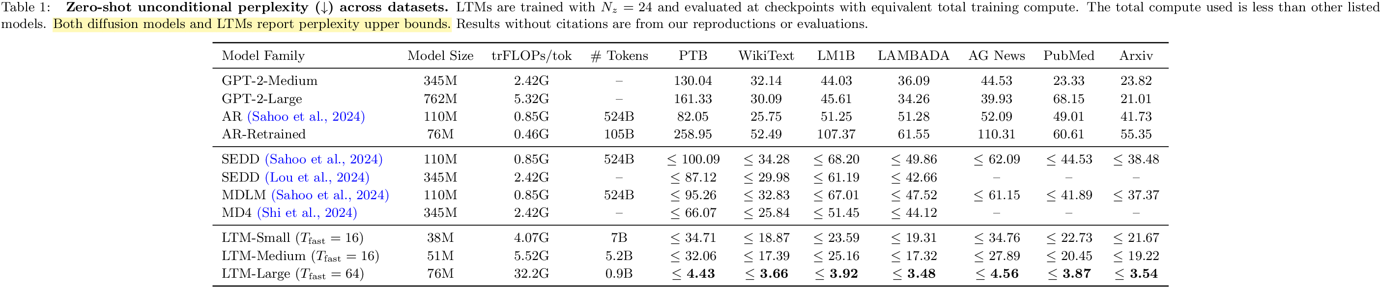
The method is interesting, but I think Table 1 needs to be interpreted carefully. I asked this here:
1. Sequence-specific posterior
The paper defines a sequence-specific variational posterior:
$$ q(\mathbf{z}\mid\mathbf{x}) = \mathcal{N}(\boldsymbol{\mu}, \boldsymbol{\sigma}^{2}) $$These are local parameters optimized for each sequence. If evaluation also performs posterior inference on the whole sequence \(\mathbf{x}\), then \(\mathbf{z}\) necessarily absorbs information from that whole sequence.
2. Upper bound, not strict AR perplexity
The caption of Table 1 already says that LTMs report perplexity upper bounds. That matters a lot. It means the paper itself is signaling that this number is not directly the same object as standard autoregressive next-token perplexity.
The released code reinforces this reading. In evaluation, it first optimizes the latent posterior for the current batch and then computes
$$ \mathrm{PPL}_{\text{LTM}} = \exp\!\left(\frac{\text{NLL} + \mathrm{KL}}{\text{sequence length}}\right), $$which is derived from the negative ELBO, not from a strict left-to-right autoregressive likelihood. Concretely, the path is essentially train_ltm.py -> posterior_optimizer_test.step() -> model.elbo(): optimize \((\mu,\log \sigma^2)\) on the sequence, then convert NLL + KL into perplexity.
Personal Note
if you want to spend extra test-time compute on latent reasoning, one way to do it is to explicitly write down latent variables, a posterior family, an ELBO, and an inner-loop inference procedure.
From that angle, LTM is a useful, more explicit, more probabilistic reference model for thinking about HRM [2]
Hierarchical Reasoning Model
G. Wang, J. Li, Y. Sun, X. Chen, C. Liu, Y. Wu, M. Lu, S. Song, Y. Abbasi Yadkori, (2025)
DOI
. and TRM [3]
Less is More: Recursive Reasoning with Tiny Networks
A. Jolicoeur-Martineau, (2025)
DOI
.