TL;DR: Exact-ZOH replaces Parcae's Euler input gain with the held-input integral for the same full-matrix write. It lowers validation loss in completed matched 140M controls and in a completed 370M paper-style follow-up. Downstream readout remains mixed: CORE Extended is higher for ZOH at both 140M and 370M, while CORE is slightly lower.
Introduction and Background
Loop models reuse weights across depth instead of using a fresh Transformer block at every layer. This makes depth an iterative computation: the model spends more serial compute while keeping the parameter count relatively small. Parcae is a recent looped language model in this line [1]
Parcae: Scaling Laws For Stable Looped Language Models
H. Prairie, Z. Novack, T. Berg-Kirkpatrick, D. Fu, (2026)
Link
. Following the prelude–recurrent–coda structure used in Huginn-style recurrent-depth models [2]
Scaling up Test-Time Compute with Latent Reasoning: A Recurrent Depth Approach
J. Geiping, S. McLeish, N. Jain, J. Kirchenbauer, S. Singh, B. Bartoldson, B. Kailkhura, A. Bhatele, T. Goldstein, (2025)
Link
, Parcae first maps the token sequence to a prelude representation \(e\), repeatedly refines a loop-depth state \(h_t\) with a recurrent Transformer branch, and then maps the final state to logits with a coda.
The central issue is stability. Repeated residual updates can make the loop state explode and produce loss spikes. Parcae frames the loop as a dynamical system over the residual stream and adds a diagonal linear control path around the recurrent branch. Abstractly, one loop step is1
$$ h_{t+1}=\bar A h_t+\bar B e+\bar{\mathcal R}(h_t,e). $$Here \(\bar A\) controls state carry-over, \(\bar B e\) writes the prelude representation back into the loop state, and \(\bar{\mathcal R}\) is the recurrent Transformer contribution. Parcae’s stabilization mostly enters through the design of \(\bar A\): it starts from a stable continuous-time generator and discretizes it exactly. That design is what makes the next mismatch visible. The state carry-over is already treated as a continuous-time object; the input write \(\bar B e\) is still implemented with an Euler gain.
To control the spectral norm, Parcae makes the homogeneous state path decay by construction. It parameterizes \(\bar A\) through an exact exponential state decay, starting from
$$ A = -\operatorname{Diag}(a), \quad a_i > 0, $$and is discretized as
$$ \bar A = \exp(\Delta A) = \operatorname{Diag}(\exp(-\Delta a_i)). $$Derivations
The diagonal control path means each state channel can be read as an independent homogeneous ODE. For channel \(i\), ignore the input write and recurrent Transformer residual for a moment:
$$ \frac{d h_i(\tau)}{d\tau}=-a_i h_i(\tau),\qquad a_i>0. $$The solution has the form
$$ h_i(\tau)=C\exp(-a_i\tau). $$The initial state fixes \(C=h_i(0)\), so after one loop step of length \(\Delta\),
$$ h_i(\Delta)=\exp(-\Delta a_i)h_i(0). $$Stacking all channels gives the Parcae carry-over operator
$$ \bar A=\operatorname{Diag}\!\left(\exp(-\Delta a_i)\right) =\exp(\Delta A),\qquad A=-\operatorname{Diag}(a). $$Every carry-over eigenvalue is therefore in \((0,1)\). This is the exact continuous-to-discrete solution for the homogeneous state path.
Thus the carry-over eigenvalues are inside the unit interval, matching the stability goal of the control path. The input write in the current implementation uses an Euler gain:
$$ h_{t+1}=\exp(-\Delta a)\odot h_t + \Delta B e + \bar{\mathcal R}(h_t,e). $$Here Euler gain means the input vector \(Be\) is multiplied by the step length \(\Delta\). It is the first-order discretization of the input integral: over a small step, the input is treated as if it contributes \(Be\) uniformly for \(\Delta\) units of loop-depth time, with the state decay inside the same interval ignored. We will see more details in later sections.
To answer this, the state-space sequence-model line gives useful context and insights: S4, Mamba, and Mamba-2 treat continuous-to-discrete state updates as explicit modeling choices [3,4,5]
Efficiently Modeling Long Sequences with Structured State Spaces
A. Gu, K. Goel, C. R\'e, (2022)
LinkMamba: Linear-Time Sequence Modeling with Selective State Spaces
A. Gu, T. Dao, (2023)
LinkTransformers are SSMs: Generalized Models and Efficient Algorithms Through Structured State Space Duality
T. Dao, A. Gu, (2024)
Link
. Mamba-style selective SSMs use this lens inside sequence-time state spaces and make quantities such as \(B\), \(C\), and \(\Delta\) token-dependent.

Continuous-to-discrete notation from the SSM line. The ZOH rule maps continuous parameters \((A,B)\) to discrete parameters \((\bar A,\bar B)\); below I specialize the same held-input formula to Parcae’s diagonal loop-depth control path.
Parcae borrows the same continuous-to-discrete language for loop depth: it uses a ZOH discretization for the state path and an Euler discretization for the input path.
However, the paper’s stability argument is primarily about the state transition \(A\) and the recurrent-state norm; the input path is left full-matrix and stabilized by normalizing the prelude output. In this post, we keep that full-matrix input-write \(B\) and change the held-input discretization.
We propose an intervention that changes only the coefficient multiplying the write vector \(Be\):
$$ \underbrace{\Delta}_{\text{Euler gain}} B e \quad\longrightarrow\quad \underbrace{\frac{1-\exp(-\Delta a)}{a}}_{\text{Exact-ZOH gain}}\odot B e. $$More details below.
From Euler Write to Exact-ZOH Write
We start from the continuous-to-discrete notation used in structured state-space model papers. S4
Introduces the structured state-space parameter-to-kernel view used for long sequence modeling.
introduced this parameter-to-kernel view for long sequence modeling [3]
Efficiently Modeling Long Sequences with Structured State Spaces
A. Gu, K. Goel, C. R\'e, (2022)
Link
, and Mamba
Reviews the ZOH discretization rule in Section 2, Eq. (4), then makes SSM parameters input-dependent.
reviews the zero-order-hold discretization explicitly in Section 2, Eq. (4) [4]
Mamba: Linear-Time Sequence Modeling with Selective State Spaces
A. Gu, T. Dao, (2023)
Link
. A continuous linear state space has the form
Under a zero-order hold (ZOH), the input is assumed constant inside one step:
$$ u(t)=u_k \qquad \text{for } t\in[k\Delta,(k+1)\Delta). $$The standard ZOH discretization is then written as
$$ \bar A=\exp(\Delta A), \qquad \bar B=(\Delta A)^{-1}\left(\exp(\Delta A)-I\right)\Delta B. $$This formula is explicitly reviewed in the Mamba paper’s Section 2 as the ZOH discretization rule for structured SSMs, where it appears as Eq. (4) [4]
Mamba: Linear-Time Sequence Modeling with Selective State Spaces
A. Gu, T. Dao, (2023)
Link
. The extra \(\Delta\) next to \(B\) is only algebraic packaging: when \(A\) is invertible,
so the same input operator can be written as
$$ \bar B=A^{-1}\left(\exp(\Delta A)-I\right)B. $$The remaining question is where the input operator \(A^{-1}(\exp(\Delta A)-I)B\) comes from.
To see this, shift step \(k\) to local time \(r=t-k\Delta\in[0,\Delta]\). With held input \(u_k\), the ODE inside this one step is
$$ \frac{d h(r)}{dr}=Ah(r)+Bu_k, \qquad h(0)=h_k. $$Multiply by the integrating factor \(\exp(-rA)\).2 Since \(A\) commutes with \(\exp(rA)\),
$$ \frac{d}{dr}\left(\exp(-rA)h(r)\right) =\exp(-rA)B u_k. $$Integrating from \(0\) to \(\Delta\) gives
$$ \exp(-\Delta A)h(\Delta)-h_k =\int_0^\Delta \exp(-sA)B u_k\,ds. $$Multiplying by \(\exp(\Delta A)\) gives the one-step solution
$$ h_{k+1}=h(\Delta)=\exp(\Delta A)h_k+ \int_0^\Delta \exp((\Delta-s)A)B u_k\,ds. $$This is the variation-of-constants form: the old state is propagated for the full step, while input written at inner time \(s\) is propagated only for the remaining time \(\Delta-s\). Set \(\tau=\Delta-s\). Then \(ds=-d\tau\), and the input integral becomes
$$ \begin{aligned} \int_0^\Delta \exp((\Delta-s)A)B u_k\,ds &=\left(\int_0^\Delta \exp(\tau A)\,d\tau\right)B u_k. \end{aligned} $$Assuming \(A\) is invertible, the antiderivative is where the \(A^{-1}\) term enters. Since
$$ \frac{d}{d\tau}\left(A^{-1}\exp(\tau A)\right) =A^{-1}A\exp(\tau A)=\exp(\tau A), $$we get
$$ \int_0^\Delta \exp(\tau A)\,d\tau =A^{-1}\left(\exp(\Delta A)-I\right). $$Therefore the discrete held-input operator is
$$ \bar B u_k=A^{-1}\left(\exp(\Delta A)-I\right)B u_k. $$Now specialize the same formula to Parcae. The loop-depth input is the prelude representation, so \(u_k=e\). The stable generator is diagonal,
$$ A=-\operatorname{Diag}(a),\qquad a_i>0, $$and the write vector before the scalar gain is \(v=Be\). Since
$$ A^{-1}=-\operatorname{Diag}(a^{-1}), \qquad \exp(\Delta A)=\operatorname{Diag}(\exp(-\Delta a)), $$the ZOH input operator acts channelwise:
$$ \begin{aligned} A^{-1}\!\left(\exp(\Delta A)-I\right)v &=-a^{-1}\odot(\exp(-\Delta a)-1)\odot v \\[0.75em] &=\frac{1-\exp(-\Delta a)}{a}\odot v \\[0.75em] &=\frac{1-\exp(-\Delta a)}{a}\odot (B e). \end{aligned} $$This gives the exact-ZOH Parcae update for the linear control path:
$$ h_{t+1}=\exp(-\Delta a)\odot h_t+ \frac{1-\exp(-\Delta a)}{a}\odot B e+ \bar{\mathcal R}(h_t,e). $$The gain also gives a simple intuition. For every \(a_i>0\),
$$ 0 < \frac{1-\exp(-\Delta a_i)}{a_i} \le \Delta. $$Equivalently,
$$ \frac{g_{\mathrm{zoh},i}}{\Delta} =\frac{1-\exp(-\Delta a_i)}{\Delta a_i}\in(0,1]. $$Euler treats within-step decay as zero. ZOH writes through the decay kernel, so fast-decay channels receive smaller writes.
As mentioned previously, here is a more concrete comparison between Exact-ZOH and Euler; the latter is the first-order approximation of the same input integral:
$$ \int_0^\Delta \exp(\tau A)d\tau =\Delta I+\frac{\Delta^2}{2}A+O(\Delta^3). $$Keeping only the first term gives the current Euler write, \(\Delta Be\). Exact-ZOH keeps the same full-matrix \(B\) parameterization and uses the held-input integral induced by Parcae’s already exact state decay.
Full-matrix \(B\): a useful interpretation
For a fixed \(a\) and \(\Delta\), the full-matrix case can be viewed as a row-rescaling of the write matrix:
$$ g_{\mathrm{zoh}}\odot Be =\operatorname{Diag}(g_{\mathrm{zoh}})Be. $$An Euler-form write can represent the same operator by choosing
$$ B'=\operatorname{Diag}\!\left(\frac{g_{\mathrm{zoh}}}{\Delta}\right)B, \qquad \Delta B'e=g_{\mathrm{zoh}}\odot Be. $$The accompanying code checks this row-rescaling identity on random full-matrix writes. The experiments below then test the training path induced by this formulation.
Implementation and cost
Numerically, the stable implementation should avoid subtractive cancellation when \(\Delta a\) is small:
$$ g_{\mathrm{zoh}}=\frac{-\operatorname{expm1}(-\Delta a)}{a}. $$In this codebase, \(a=\exp(A_{\log})>0\) and \(\Delta=\operatorname{softplus}(\mathrm{dt\_bias})>0\), so both the decay and the held-input gain remain positive. The forward pass computes
$$ \operatorname{decay}=\exp(-\Delta a),\qquad g_{\mathrm{zoh}}=\frac{-\operatorname{expm1}(-\Delta a)}{a}. $$Cost
The change is almost cost-free at model scale. The full-matrix \(B\) parameterization is unchanged, so the write \(Be\) has the same \(O(d^2)\) cost and the same parameter count. Exact-ZOH replaces the scalar step gain \(\Delta\) with a channelwise gain and then multiplies \(g_{\mathrm{zoh}}\odot (Be)\). Computing this gain costs \(O(d)\) elementwise work per loop step, or it can be cached whenever \(\Delta\) and \(a\) are unchanged during a forward pass. Relative to the recurrent Transformer branch and the existing full-matrix write, the added cost is negligible; the intervention adds no parameters and no extra recurrent block.
Experiments and Results
Does the exact zero-order-hold input gain improve over the Euler input gain in real experiments?
We compare those two methods under controlled budgets and tuned hyperparameters. For each matched pair, the architecture, recurrent Transformer branch, recurrence budget, data recipe, optimizer recipe, and full-matrix \(B\) parameterization family are matched; only the input-write gain formula changes. 3
Protocol
The main completed comparisons use the Parcae-small (140M) model family and the same language-modeling validation stream. I use two 140M recipes because they answer different questions, then add one completed Parcae-medium (370M) paper-style follow-up to check whether the validation-loss direction survives at the next scale.
- The fixed no-stochastic-depth (no-SD) probe removes stochastic depth, uses fixed recurrence with per-batch iteration, Adam
2e-3, Muon8e-3, and a constant schedule, which is selected through a sweep over learning rates and optimizer settings. This recipe isolates the input-gain change with minimal recurrence sampling noise. - The paper-style recipe follows the original Parcae stochastic recurrence contract:
poisson-truncated-fullsampling over recurrence depth, and apply per-sequence recurrence which means each sequence in the batch can have a different recurrence depth; Adam/Muon8e-3/8e-3, and trapezoid cooldown0.5. This is the stricter recipe for the long-run comparison.
The direct metric is validation loss on the same language-modeling validation stream. The 0.2B and 0.5B matched pairs are short-budget formulation probes: they ask whether the input-gain change has the right sign under controlled recipes. The completed 11.2B paper-style pair is the main 140M long-run comparison. The completed 29.6B 370M pair is a scale follow-up: it tests whether the sign persists under the medium Parcae paper-style contract.
| Branch | Role | Budgets | Recipe status |
|---|---|---|---|
| Fixed no-SD | Formulation probe | 0.2B, 0.5B | Tuned LR/optimizer probe; no stochastic depth |
| Paper-style probe | Recipe compatibility check | 0.2B, 0.5B | Original stochastic recurrence contract |
| Paper-style long run | Main 140M completed comparison | 11.2B | Original stochastic recurrence contract |
| Paper-style scale check | 370M completed follow-up | 29.6B | Original stochastic recurrence contract; Parcae-medium |
I also report downstream evaluation for the completed paper-style long pairs. The downstream panels follow the DataComp-LM / DCLM evaluation idea [6]
DataComp-LM: In search of the next generation of training sets for language models
J. Li, A. Fang, G. Smyrnis, M. Ivgi, M. Jordan, S. Gadre, H. Bansal, E. Guha, S. Keh, K. Arora, S. Garg, R. Xin, N. Muennighoff, others, (2024)
Link
: task accuracies are centered against random-baseline performance before aggregation, so random-level performance maps to 0 and higher is better. The evaluator reports the CORE and CORE Extended aggregates below in this centered-score convention. CORE is the 22-task panel used as the lower-variance downstream check; CORE Extended is a broader 46-task panel that adds MMLU, SIQA, additional BigBench tasks, math and logical reasoning, reading and reasoning exams, PubMedQA, and safety/bias tasks. These downstream panels serve as capability checks for the completed paper-style long pairs; validation loss remains the selection metric for the short-budget probes.
Validation Loss
| Setting | Tokens | Euler val ↓ | ZOH val ↓ | Δ val ↓ |
|---|---|---|---|---|
| Fixed no-SD probe | 0.2B | 4.1022 | 4.0859 | -0.0163 |
| Fixed no-SD probe | 0.5B | 3.6761 | 3.6710 | -0.0051 |
| Paper-style probe | 0.2B | 4.2940 | 4.2750 | -0.0190 |
| Paper-style probe | 0.5B | 3.6357 | 3.6233 | -0.0124 |
| Paper-style long run | 11.2B | 2.9291 | 2.9140 | -0.0151 |
| Paper-style scale check, 370M | 29.6B | 2.6397 | 2.6386 | -0.0011 |
The validation-loss result is consistent across the completed matched pairs. The short-budget rows show that the formulation change is directionally positive under both fixed no-SD and paper-style recipes. The main 11.2B paper-style run gives the completed 140M long-run comparison: Euler/full-matrix finishes at 2.9291, while Exact-ZOH/full-matrix finishes at 2.9140. The completed 370M paper-style follow-up keeps the sign but with a much smaller gap: Euler/full-matrix finishes at 2.6397, while Exact-ZOH/full-matrix finishes at 2.6386.
As a reproduction sanity check, the Euler/full-matrix paper-style baseline is close to the original Parcae small reference. The Parcae paper reports 140M Parcae at Val. PPL = 19.06, or ln(PPL) = 2.9476, after the same 11.2B token budget [1]
Parcae: Scaling Laws For Stable Looped Language Models
H. Prairie, Z. Novack, T. Berg-Kirkpatrick, D. Fu, (2026)
Link
. Our matched Euler/full-matrix run is slightly better on validation loss (2.9291), so the baseline is at least as strong as the paper reference on the language-modeling objective. Its downstream CORE numbers are in the same range and a bit lower: the paper reports about 0.1404 CORE and 0.0967 CORE Extended in the decimal convention used here, while our Euler/full-matrix checkpoint reports 0.1353 and 0.0876, still within reasonable range.

Paper-style 11.2B validation curves with a tail zoom. Both runs keep the Parcae stochastic recurrence contract and full-matrix write parameterization matched; ZOH changes only the input-gain formula and finishes at lower validation loss.
Downstream CORE Readout
For the completed 11.2B paper-style pair, the downstream readout is mixed. Exact-ZOH has lower validation loss and a slightly higher CORE Extended score, while Euler remains slightly ahead on the smaller 22-task CORE aggregate. This is why the downstream statement here is deliberately narrower than the validation-loss statement: Exact-ZOH improves the language-modeling objective, and the downstream panels give a mixed but encouraging readout.
1234, 2345, 3456 and the same downstream evaluator; the CORE column is the 22-task subset aggregate, while CORE Extended is the broader 46-task aggregate. ZOH improves validation and CORE Extended, while Euler remains slightly ahead on CORE.| Input write | Validation loss ↓ | CORE ↑ | CORE Extended ↑ |
|---|---|---|---|
| Euler full-matrix | 2.9291 | 0.1353 ± 0.0008 | 0.0876 ± 0.0006 |
| Exact-ZOH full-matrix | 2.9140 | 0.1313 ± 0.0025 | 0.0911 ± 0.0010 |
| Δ ZOH - Euler | -0.0151 | -0.0040 | +0.0035 |
CORE and CORE Extended category definitions used in the radar plot
The 11.2B paper-style radar averages centered task scores within each category below. Short-budget CORE numbers are omitted here because those runs probe the formulation; downstream capability is better demonstrated by the completed long-run pair.
CORE 22-task panel. The left radar uses the original 22-task CORE suite grouped into nine finer categories:
- Commonsense continuation 2 tasks:
hellaswag_zeroshot,hellaswag. Narrative-ending plausibility with zero-shot and few-shot HellaSwag. - Factual QA 2 tasks:
jeopardy,bigbench_qa_wikidata. Exact factual recall through Jeopardy-style and Wikidata QA prompts. - Science QA 3 tasks:
arc_easy,arc_challenge,openbook_qa. School-science knowledge and light inference. - Commonsense reasoning 3 tasks:
copa,commonsense_qa,piqa. Everyday causal, physical, and affordance reasoning. - Cloze LM 1 task:
lambada_openai. Exact continuation from broad passage context. - Schema/coreference 2 tasks:
winograd,winogrande. Pronoun and schema-style semantic disambiguation. - Formal/symbolic 5 tasks:
bigbench_dyck_languages,agi_eval_lsat_ar,bigbench_cs_algorithms,bigbench_operators,bigbench_repeat_copy_logic. Structured symbolic manipulation, algorithms, and verbal logic. - Reading QA 3 tasks:
squad,coqa,boolq. Question answering from supplied passages and yes/no context. - Language identification 1 task:
bigbench_language_identification. Language identification among candidate labels.
CORE Extended 46-task panel. The right radar uses the broader CORE Extended suite grouped into six evaluator families:
- Language understanding 8 tasks:
hellaswag_zeroshot,lambada_openai,hellaswag,winograd,winogrande,bigbench_language_identification,bigbench_conlang_translation,bigbench_conceptual_combinations. - World knowledge 7 tasks:
jeopardy,bigbench_qa_wikidata,arc_easy,arc_challenge,mmlu_zeroshot,mmlu_fewshot,bigbench_misconceptions. - Commonsense 8 tasks:
copa,commonsense_qa,piqa,openbook_qa,siqa,bigbench_novel_concepts,bigbench_strange_stories,bigbench_strategy_qa. - Symbolic/math 11 tasks:
bigbench_dyck_languages,agi_eval_lsat_ar,bigbench_cs_algorithms,bigbench_operators,bigbench_repeat_copy_logic,bigbench_elementary_math_qa,bigbench_logical_deduction,simple_arithmetic_nospaces,simple_arithmetic_withspaces,math_qa,logi_qa. - Reading 8 tasks:
squad,coqa,boolq,pubmed_qa_labeled,agi_eval_lsat_rc,agi_eval_lsat_lr,bigbench_understanding_fables,agi_eval_sat_en. - Safety/bias 4 tasks:
winogender_mc_female,winogender_mc_male,enterprise_pii_classification,bbq.
For the radar figure, CORE Extended is grouped more coarsely because the added tasks are heterogeneous. Each axis averages the centered scores of the tasks assigned to that evaluator family.

CORE and CORE Extended category profiles for the completed paper-style 11.2B pair. The left panel uses the 22-task CORE suite grouped into the nine categories listed above; the right panel uses the 46-task CORE Extended suite grouped by evaluator family. Both panels use centered task scores on the same radial scale, where 0 is random-baseline performance and higher is better.
370M Paper-Style Scale Follow-Up
After the 140M paper-style result, I ran the same full-matrix Euler/ZOH comparison at Parcae-medium scale. The 370M follow-up uses the medium paper-style contract: fixed full-matrix input writes, r8/b4 recurrence, poisson-truncated-full stochastic recurrence, per-sequence iteration, WBS/MBS 256/16, Adam/Muon 8e-3/8e-3, trapezoid cooldown 0.5, and a 29.6B token budget. Both runs finish at the same final checkpoint step, and downstream readouts use the same CORE Extended evaluator with seeds 1234, 2345, and 3456.
| Input write | Validation loss ↓ | CORE ↑ | CORE Extended ↑ |
|---|---|---|---|
| Euler full-matrix | 2.6397 | 0.2033 ± 0.0006 | 0.1284 ± 0.0035 |
| Exact-ZOH full-matrix | 2.6386 | 0.1982 ± 0.0012 | 0.1337 ± 0.0019 |
| Δ ZOH - Euler | -0.0011 | -0.0051 | +0.0053 |
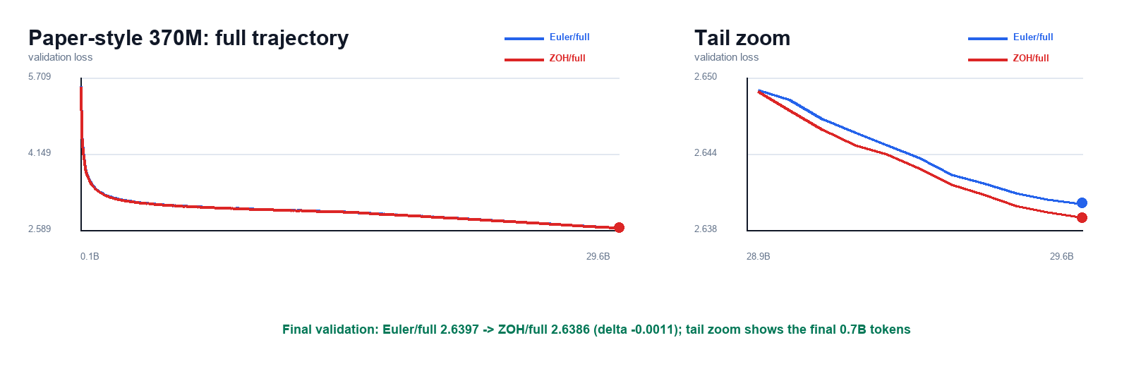
Paper-style 370M validation curves with a tighter tail zoom over the final 0.7B tokens. Both runs keep the Parcae-medium stochastic recurrence contract and full-matrix write parameterization matched; ZOH changes only the input-gain formula and finishes slightly lower on validation loss.
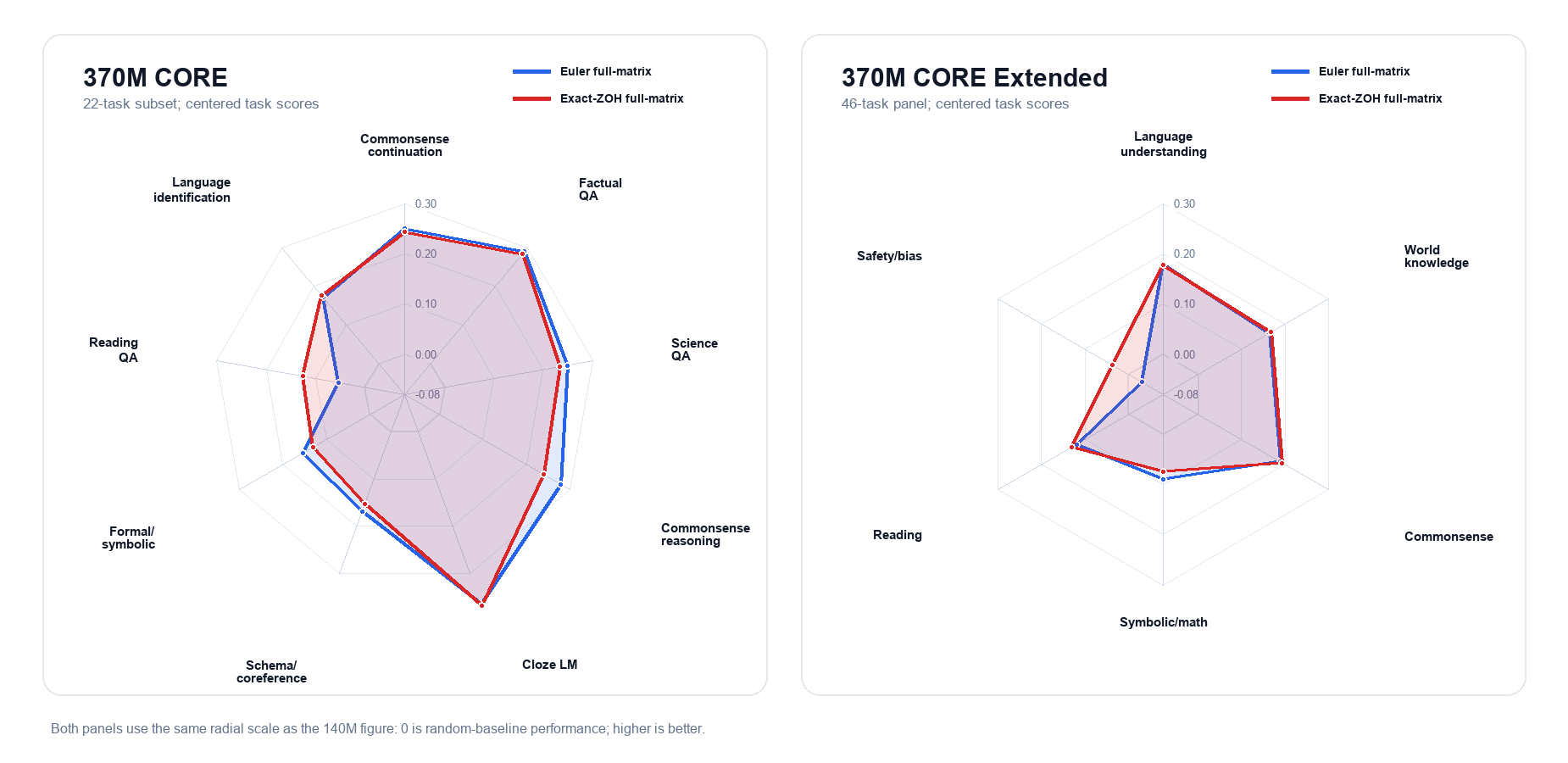
CORE and CORE Extended category profiles for the completed paper-style 370M pair. The left panel uses the 22-task CORE subset; the right panel uses the 46-task CORE Extended suite grouped by evaluator family. Both panels use centered task scores on the same radial scale as the 140M radar.
The 370M result is useful because it is matched and complete, not because it is dramatic. It says the validation-loss direction survives the medium-scale paper-style contract. It also keeps the downstream story honest: the broader CORE Extended panel moves toward ZOH, while the smaller CORE aggregate remains better for Euler.
Summary
Across completed matched Parcae full-matrix controls, replacing the Euler input gain with the exact-ZOH gain lowers validation loss, including the paper-style 11.2B 140M run and the paper-style 29.6B 370M follow-up. The 370M validation gap is small, so I read it as sign consistency rather than a large scale-up win. Downstream evaluation is more nuanced: Exact-ZOH improves CORE Extended slightly at both scales, while Euler remains slightly ahead on the smaller CORE aggregate. I therefore treat Exact-ZOH as a clean validation-loss improvement to Parcae’s control path, with downstream effects that still need larger-scale confirmation.
Appendix
Code and Reproducibility
- Code fork: github.com/huskydoge/parcae-zoh-exact.
- Implementation entry point:
parcae_lm/modules/injection.py. - Patch-level checks:
tests/test_exact_zoh_injection.py. - Reference numbers:
results/exact_zoh_full_matrix_results.csv.
Other Loop Mechanisms
The ZOH result above changes the discretization of Parcae’s input write. During the same investigation, recent Hyperloop Transformers work [7]
Hyperloop Transformers
A. Zeitoun, L. Torroba-Hennigen, Y. Kim, (2026)
Link
motivated a second check: can extra loop-state connectivity improve raw recurrence, and does it still help once Parcae’s stabilizing control path is already present? That question also made me revisit Kimi’s Attention Residuals [8]
Attention Residuals
Kimi Team, (2026)
Link
, which suggested a related residual-history variant. I tested both mechanisms as appendix context for the main ZOH claim.
I use PLC here to mean Parcae’s linear control path: the diagonal stable carry-over \(\bar A\) and input write \(\bar B e\) wrapped around the recurrent Transformer branch. The contrast is between two families:
- Raw-loop family: the recurrent Transformer is looped with the Parcae diagonal control path absent.
- PLC family: the same mechanisms are added on top of the Parcae diagonal control path.
The mechanism variants are Loop AttnRes, our loop-depth adaptation of Attention Residuals [8]
Attention Residuals
Kimi Team, (2026)
Link
, and HyperConnectedLoop, our Hyperloop-style adaptation of loop-level hyper-connections [7]
Hyperloop Transformers
A. Zeitoun, L. Torroba-Hennigen, Y. Kim, (2026)
Link
. Hyperloop-style connections are attractive because they add extra loop-state mixing with relatively small parameter overhead; Loop AttnRes asks a related question from the residual-history side, replacing fixed residual accumulation with a learned aggregation over loop-history residuals.
The base raw loop and the Parcae-controlled loop can be written schematically as
$$ \begin{aligned} \text{raw loop:}\qquad h_{t+1} &= h_t + \mathcal R_\theta(h_t,e),\\ \text{PLC / Parcae:}\qquad h_{t+1} &= \bar A h_t + \bar B e + \mathcal R_\theta(h_t,e). \end{aligned} $$The two appendix mechanisms modify the loop-state update around \(\mathcal R_\theta\). They are useful context for the ZOH result because they ask whether extra residual-history machinery can substitute for, or add to, the stabilizing PLC path.
Mechanism sketches: Loop AttnRes and HyperConnectedLoop
- Loop AttnRes. Let the recurrent branch propose \(u_t=\mathcal R_\theta(h_t,e)\) and define the raw loop delta \(\Delta_t=u_t-h_t\). The implementation stores the initial state and previous deltas, \(V_t=[h_0,\Delta_0,\ldots,\Delta_t]\), then uses a learned loop-depth query \(q_t\) to score RMS-scaled history values: \[ \alpha_t=\operatorname{softmax}\!\left(q_t^\top \operatorname{RMSNorm}(V_t)\right), \qquad h_{t+1}=\sum_i \alpha_{t,i}V_{t,i}. \] In the PLC version, the same aggregation is applied after the Parcae core proposal. The question is whether learned selection over loop-history residuals is better than simply taking the newest loop proposal.
- HyperConnectedLoop. The implemented Hyperloop-style variant keeps \(K\) loop streams \(S_t^{(1:K)}\). A gate network reads the RMS-normalized flattened streams and produces per-stream diagonal pre, post, and residual gates: \[ a_t=\sigma(W_t^{\mathrm{pre}}z_t+b_t^{\mathrm{pre}}),\quad b_t=2\sigma(W_t^{\mathrm{post}}z_t+b_t^{\mathrm{post}}),\quad r_t=\sigma(W_t^{\mathrm{res}}z_t+b_t^{\mathrm{res}}). \] The pre-gate mixes the streams into the recurrent-branch input, the post-gate writes the branch output back into each stream, and the residual gate carries stream memory: \[ c_t=\sum_k a_{t,k}S_t^{(k)},\qquad u_t=\mathcal R_\theta(c_t,e),\qquad S_{t+1}^{(k)}=r_{t,k}S_t^{(k)}+b_{t,k}(u_t+p_t). \] The exposed recurrent state is the stream mean, \(h_{t+1}=K^{-1}\sum_k S_{t+1}^{(k)}\). This is a loop-level Parcae adaptation with diagonal per-stream gates and mean readout.
| Family | Mechanism | Val loss ↓ | Δ vs raw ↓ | CORE ↑ |
|---|---|---|---|---|
| Raw loop | none | 3.7862 | 0.0000 | 0.0513 ± 0.0018 |
| Raw loop | Loop AttnRes | 3.7741 | -0.0121 | 0.0468 ± 0.0013 |
| Raw loop | HyperConnectedLoop | 3.6913 | -0.0949 | 0.0459 ± 0.0026 |
| PLC / Parcae | diagonal control | 3.6761 | -0.1101 | 0.0618 ± 0.0020 |
The raw-loop table shows that the mechanisms are meaningful. HyperConnectedLoop gives a large language-modeling improvement over the raw loop, and Loop AttnRes also moves in the right direction on validation loss. The stabilized Parcae control path is the stronger intervention in this matrix: it beats the raw-loop mechanisms on final validation loss and aggregate CORE.
The second check asks whether those same mechanisms still help once the PLC path is already present. This is the harder comparison, because the baseline is no longer an unstable raw loop; it is already Parcae’s controlled loop.
| PLC-family variant | 200M best val ↓ | 500M val ↓ | Δ vs base ↓ | CORE ↑ |
|---|---|---|---|---|
| Parcae base | 4.1927 | 3.6787 | 0.0000 | 0.0505 ± 0.0039 |
| + Loop AttnRes | 4.1364 | 3.7043 | +0.0256 | 0.0408 ± 0.0014 |
| + HyperConnectedLoop | 4.1223 | 3.7123 | +0.0335 | 0.0440 ± 0.0013 |
This appendix gives a useful boundary for the main result. Hyperloop-style connections and loop-history residual aggregation can improve a raw loop, while the tuned Parcae diagonal-control baseline stays ahead once that stabilizing path is present. The practical lesson is that stabilization is the first-order control surface: before PLC, extra loop mechanisms help; after PLC, the simpler controlled base stays stronger in this matrix. Exact-ZOH then improves that control surface by making the input write consistent with the exact state decay.
Limitations and Future Work
This post is more like a formulation and validation check. The completed 370M follow-up is directionally consistent on validation loss, but a full scaling-law claim still needs more seeds, 770M-scale checks, and broader downstream confirmation.
Another useful direction is the interaction between residual control and normalization. The experiments here use the current pre-norm Parcae implementation. It would be natural to test whether the same input-write discretization behaves differently under post-norm, residual normalization, or other normalization choices inside the recurrent Transformer branch.
References
H. Prairie, Z. Novack, T. Berg-Kirkpatrick, D. Fu, (2026)
Link
J. Geiping, S. McLeish, N. Jain, J. Kirchenbauer, S. Singh, B. Bartoldson, B. Kailkhura, A. Bhatele, T. Goldstein, (2025)
Link
T. Dao, A. Gu, (2024)
Link
J. Li, A. Fang, G. Smyrnis, M. Ivgi, M. Jordan, S. Gadre, H. Bansal, E. Guha, S. Keh, K. Arora, S. Garg, R. Xin, N. Muennighoff, others, (2024)
Link
Parcae explicitly includes the nonlinear recurrent Transformer contribution \(\bar{\mathcal R}\), then removes it in a linear approximation to expose an analytically tractable discrete LTI control path over the residual state. This is an analytical lens, not a claim that the Transformer residual branch is absent or harmless. Their empirical claim is narrower: instability in prior looped architectures is associated with large spectral norms in the injection parameters under this control-path view. The ZOH change here applies to that same linear input path while leaving the recurrent Transformer branch unchanged. [1] Parcae: Scaling Laws For Stable Looped Language Models
H. Prairie, Z. Novack, T. Berg-Kirkpatrick, D. Fu, (2026)
Link ↩︎This is the standard integrating-factor trick: choose a multiplier that turns the left-hand side of a linear forced ODE into an exact derivative. Very elegant one! ↩︎
For the fixed no-SD probing branch, I first swept learning-rate and optimizer settings, then reported the matched Euler/ZOH pair under the selected recipe. I treat this branch as a formulation probe; the paper-style long run carries the final statistical claim in this post. ↩︎
Cited as
Use the plain citation or copy the BibTeX entry below.
Benhao Huang. (Apr 2026). Exact Input Writes Improve Stable Looped Language Models. Husky's Log. /husky-blog/posts/recursive_models/improve-parcae/
@article{huang2026exact,
  title   = "Exact Input Writes Improve Stable Looped Language Models",
  author  = "Benhao Huang",
  journal = "Husky's Log",
  year    = "2026",
  month   = "Apr",
  url     = "https://huskydoge.github.io/husky-blog/posts/recursive_models/improve-parcae/"
}