The Long-Term Decay Property of RoPE

Introduction

RoPE¹ is the most common positional embedding method that has been applied in many popular Language Models. RoPE has several properties, among which the long-term decay property is really interesting. Recently, I've been researching on how to make long-term decay property more customizable and controllable. Therefore, I want to get myself really understand why RoPE has the long-term decay property and how it works. In this post, I try to provide a more intuitive understanding of the long-term decay property of RoPE, and will also cover some recent researches relevant to RoPE.

Review | Some Details

Before getting the proof, let's first recal the Long-term decay of RoPE (Sec.3.4.3) in the original paper¹. Contents below are completely copied from the orginal paper, the equation number from paper is kept.

We can group entries of vectors $\boldsymbol{q}=\boldsymbol{W}_q \boldsymbol{x}_m$ and $\boldsymbol{k}=\boldsymbol{W}_k \boldsymbol{x}_n$ in pairs, and the inner product of RoPE in Equation (16) can be written as a complex number multiplication.

where $\boldsymbol{q}_{[2 i: 2 i+1]}$ represents the $2 i^{\text {th }}$ to $(2 i+1)^{\text {th }}$ entries of $\boldsymbol{q}$. Denote $h_i=\boldsymbol{q}_{[2 i: 2 i+1]} \boldsymbol{k}_{[2 i: 2 i+1]}^*$ and $S_j=$ $\sum_{i=0}^{j-1} e^{i(m-n) \theta_i}$, and let $h_{d / 2}=0$ and $S_0=0$, we can rewrite the summation using Abel transformation

Thus,

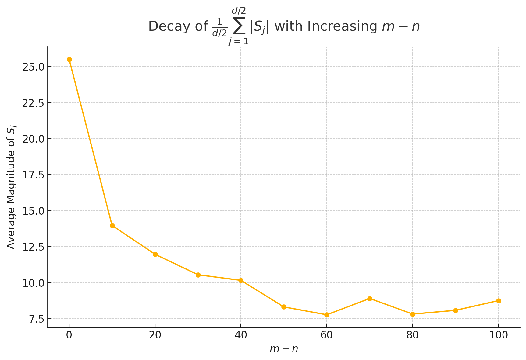
Note that the value of $\frac{1}{d / 2} \sum_{i=1}^{d / 2}\left|S_i\right|$ decay with the relative distance $m-n$ increases by setting $\theta_i=10000^{-2 i / d}$, as shown in Figure (2).

I believe some readers will have common questions with me, it seems in this part of paper, many details are elliminated for simplicity. I don't want to be the guy who just pretend these details are not important, focus on ideas, I will present more derivations here, since so far I haven't seen any detailed explanations here, including the blog of the author².

Let's revise some annotation here. $\boldsymbol{R}_{\theta, m}^d$ is the following matrix:

$\theta_i$ belongs to $\Theta=\left\{\theta_i=10000^{-2(i-1) / d}, i \in[1,2, \ldots, d / 2]\right\}$​​, where 10000 is called "base", as a predefined constant. The value of base will have interesting effect on RoPE, which we will discuss later.

$\boldsymbol{x}_i \in \mathbb{R}^d$ is the d-dimensional word embedding vector of token $w_i$ (Let $\mathbb{S}_N=\left\{w_i\right\}_{i=1}^N$ be a sequence of $N$ input tokens with $w_i$ being the $i^{t h}$ element. The corresponding word embedding of $\mathbb{S}_N$ is denoted as $\mathbb{E}_N=\left\{\boldsymbol{x}_i\right\}_{i=1}^N$). $\boldsymbol{q}=\boldsymbol{W}_q \boldsymbol{x}_m$ and $\boldsymbol{k}=\boldsymbol{W}_k \boldsymbol{x}_n$ are of the shape as $\boldsymbol{x_i}$.

Derivation of Eq.(35)

Now let's first derive Eq.(35). We first try to get its complete form without using complex numbers. Each block $\boldsymbol{R_{m\theta_i}}$ in matrix $\boldsymbol{R_{\theta, m}^d}$ is a rotation matrix, where $\boldsymbol{R_{m\theta_i}}=\left(\begin{array}{cc} \cos m \theta_1 & -\sin m \theta_1 \\ \sin m \theta_1 & \cos m \theta_1 \end{array}\right)$ means contrarotating $m\theta_1$, while

which means rotate $n\theta_i$ clockwise. Therefore, the LHS of Eq.(35) can be written as:

It's easy to see that the RHS of Eq.(4) is a scalar. We focus on $\boldsymbol{q}^T\boldsymbol{R}_{\Theta, n-m}^d$ first. For index $2j, 2j+1, 0\le j\le d/2-1$ , It's easy to see that elements $[q_{2j},q_{2j+1}]$ in $\boldsymbol{q}^T$ will only interact with the block $\boldsymbol{R_{(n-m)\theta_{j+1}}}$, and we have:

And these two elements will be multiplied with the $2j, 2j+1$ elements of $\boldsymbol{k}$, then we finally get:

Then we back to the complex number form used by authors. In Eq.(35), it's said $\boldsymbol{q}_{[2 i: 2 i+1]}\cdot k_{[2 i: 2 i+1]}$ is operated as complex multiplication, which means:

(Please don't confuse your self with the index $i$ and $i$ representing imaginary number). Then if we multiply the RHS of Eq.(5) with $e^{i(m-n)\theta_i}=cos(m-n)\theta_i+i\cdot sin(m-n)\theta_i$, and focus on real part, we will magically get the Eq.(key), with $i$ substituted by $j$. It's quite elegant!

We then sum up $j$ from $0$ to $d/2-1$, then we successfully get Eq.(35).

Derivation of Eq.(36)

The derivation of Eq.(36) is relatively simple. We just focus on $S_{i+1}$, and combine the same items will give us correct coefficient which is $h_{i+1}-h_i$. Then we sum up $i$ from $0$ to $d/2-1$, and we get Eq.(36). See Wikipedia for more details about Abel transformation.

Why Long-term Decay?

Well, then we arrive at the most important part, we try to understand why the value of $\frac{1}{d / 2} \sum_{j=1}^{d / 2}\left|S_j\right|$ decay with the relative distance $m-n$ increases by setting $\theta_i=10000^{-2 i / d}$, where $S_j=$ $\sum_{i=0}^{j-1} e^{i(m-n) \theta_i}$. This property could also be described as "the closer token gets more attention: the current token tends to pay more attention to the token that has a smaller relative distance", as discussed in Sec.4 of this paper⁴.

It's acutally very hard to analyze by taking derivative of $(m-n)$, since we cannot easily find the analytical solution of.

One intuitive way to understand is to take the sum of $e^{i(m-n)\theta_i}$ as walking on a plane, which is the geometric meaning of adding two vectors. Apparently, when $m-n$ is close to zero, then we almost walking in a constant direction, which makes the sum of $e^{i(m-n)\theta_i}$ large. However, when $m-n$ is large, then the sum of $e^{i(m-n)\theta_i}$ will be small, since we are walking in different directions, with the worst case where we are walking in a circle.

The Concept of Phase Cancellation

Phase cancellation occurs when complex exponentials (vectors on the unit circle in the complex plane) with differing directions are summed together. The result can be a vector with a smaller magnitude than the individual vectors due to the geometric addition properties of complex numbers.

The Sum $S_j$

Recall: $S_j = \sum_{i=0}^{j-1} e^{i(m-n) \theta_i}$ with $\theta_i = 10000^{-2i/d}$.

Examining the Phases

1. Distribution of Phases:

   • The phases $(m-n)\theta_i$ for each term in the sum depend on both $m-n$ and $i$.
   • As $m-n$ increases, the value of $(m-n)\theta_i$ changes more rapidly due to the exponential nature of $\theta_i$.
   • For a fixed large $m-n$, the phases $(m-n)\theta_i$ effectively "scan" a broader range of angles on the unit circle as $i$ varies.

2. Uniform Distribution Assumption:

   • If $m-n$ is sufficiently large and $i$ ranges over a significant interval, $(m-n)\theta_i$ can cover the interval $[0, 2\pi]$ multiple times, depending on $m-n$, effectively randomizing the phase angles.
   • Under this assumption, the phases of the terms in $S_j$ can be seen as being uniformly distributed across $[0, 2\pi]$.

Illustrating Cancellation

• Cancellation Through Averaging:

  • If the phases of $e^{i(m-n) \theta_i}$ are uniformly distributed or nearly so, the expected value of their sum approaches zero: $E\left[\sum_{i=0}^{j-1} e^{i(m-n) \theta_i}\right] = \sum_{i=0}^{j-1} E[e^{i(m-n) \theta_i}] = \sum_{i=0}^{j-1} \int_0^{2\pi} e^{i\phi} \frac{d\phi}{2\pi} = 0$
  • Intuitively speaking, $E[e^{i\phi}]$ over $[0, 2\pi]$ is zero because for every vector, there is another vector pointing in the opposite direction, cancelling out.

• Expected Magnitude with High Variability:

  • While the average expected value is zero, individual realizations of $S_j$ can vary widely, typically resulting in smaller magnitudes as more vectors are added due to increasing likelihood of opposite directions.
  • The more terms added (i.e., larger $j$), the greater the potential for cancellation, especially when $(m-n)\theta_i$ provides a full or multiple rotations around the circle.

Surveying

1.The Influence of Base Choice on Long-term Decay

For same $i$ and $d$, larger base will make the $\theta_i=base^{-2(i-1)/d}$ smaller. According to the blog here³, too small base (e.g. 1) will completely destroy the long-term decay property, while too large base will also decrease the long-term decay property. However, it's argued in aother work that to achieve longer context we need to have larger base⁴, more detailed results from this paper are illustrated by this table:

2. Long-term Decay of the Ability to Attend More to Similar Tokens than Random Tokens

Theorem⁴: Assuming that the components of query $q \in R^d$ and key $k \in R^d$ are independent and identically distributed, their standard deviations are denoted as $\sigma \in R$. The key $k^*=q+\epsilon$ is a token similar to the query, where $\epsilon$ is a random variable with a mean of 0 . Then we have:

3. The perplexity cannot be used to evaluate long context capabilities

As indicated in ⁴, perplexity is not a good metric to evaluate the long context capabilities of a model. In Long-Eval bench, a model with small perplexity could have very low accuracy.

Desserts

Jianlin Su is a very talented guy, his Blogs are all very insightful. Among his numerous blogs, a series called "To upgrade Transformer" (Transformer 升级之路) really deserve an In-depth reading. Here I curate a list, since the search engine in the blog website seems not to work well.

Transformer 升级之路：2、博采众长的旋转式位置编码

• This blog introduces RoPE.

Transformer升级之路：4、二维位置的旋转式位置编码

• This blog introduces 2D RoPE, which could be applied in ViT.

Transformer 升级之路：7、长度外推性与局部注意力

Transformer 升级之路：9、一种全局长度外推的新思路

Transformer 升级之路：10、RoPE 是一种 β 进制编码

Transformer升级之路：17、多模态位置编码的简单思考

Transformer 升级之路：18、RoPE 的底数选择原则

Still updating.....